Industrial generator TCO is the practical way to compare generator proposals by lifecycle cost—not only purchase price. In this guide, we break down fuel consumption, maintenance & spares, downtime risk, ATS/load shedding/paralleling scope, and FAT/SAT acceptance testing so you can choose a standby generator system that performs during real outage events.
Reviewed by: Enerzip Power Technology (Weifang) Co., Ltd. – Applications & Integration Team
Last updated: 22-Dec-2025
Update policy: This guide is reviewed when common industrial duty assumptions, fuel price dynamics, EPC control scope expectations (ATS/paralleling), or acceptance testing practices (FAT/SAT) change.
Scope: Practical lifecycle engineering for industrial generator systems (diesel / natural gas / biogas), with emphasis on reliability, downtime risk, and project-grade integration.
About the reviewing team
Enerzip Applications & Integration Team supports EPC contractors, distributors, and industrial users by translating load profiles, duty cycles, and site constraints into actionable generator configurations. We typically validate assumptions through FAT/SAT planning, staged load pick-up logic, and site airflow/cooling checks—because most real project failures happen at transfer, motor start, step load, or high-ambient operation.
Why “low price” fails as a decision rule
In industrial projects, a generator set is not a commodity box. It is a power system that must start, stabilize, accept load steps, survive high ambient temperature, and coordinate with ATS and site protection. Yet procurement often starts with a single number: purchase price.
That’s where many projects lose money. A low initial price may look attractive in a tender comparison, but lifecycle cost often tells a different story—especially when the genset is expected to protect production lines, critical pumping, cold-chain warehouses, hospitals, data centers, or process utilities.
- Higher fuel burn at the same load (worse partial-load behavior, higher L/h or higher g/kWh).
- Weaker transient response (deeper voltage/frequency dips) causing nuisance trips and repeated commissioning work.
- Reduced cooling margin (common in 40–50°C sites) leading to thermal derating or shutdowns during long runs.
- Higher maintenance burden (shorter intervals, unclear spares route, longer corrective downtime).
- Incomplete control scope (ATS logic, staged load pick-up, shedding, paralleling) shifting integration risk to the EPC.
Enerzip Field Note: Post-delivery disputes rarely start with “kW is insufficient.” They start with an undefined event: ATS transfer timing, largest motor re-acceleration after transfer, UPS/rectifier step load pick-up, or the cooling airflow path inside a canopy/container. A unit can pass a steady-state load test yet still fail at the site’s “moment of truth.”
Practical fix: Put acceptance targets into the RFQ and tie them to FAT/SAT. Example targets often used as starting points in PLC/UPS-heavy industrial sites (must be confirmed with your equipment tolerance): voltage dip ≤ 15% for ≤ 1–2 seconds during the worst motor start, and frequency dip ≤ 10% with recovery within ≤ 5 seconds after the largest step load.
In procurement reviews, industrial generator TCO is where “cheap” decisions fail, because the cost shows up later as fuel invoices, corrective maintenance, and outage-driven losses.
What Industrial Generator TCO Includes (Total Cost of Ownership)
Total cost of ownership (TCO) is the full lifecycle cost of owning and operating a generator system over a defined service life—commonly 5, 10, or 15 years. For general reference on life-cycle costing methodology, readers may also review the NIST Life-Cycle Costing Manual. For industrial sites, TCO must include both measurable costs and risk-driven costs.
- CAPEX: purchase price + logistics + installation + integration scope (ATS, switchgear, monitoring, commissioning).
- Fuel cost: consumption rate × runtime × fuel price, adjusted for duty cycle and partial-load behavior.
- Maintenance & spares: scheduled service, consumables, parts replacement, labor, and availability of service network.
- Downtime risk cost: production loss, safety risk, penalties, spoilage, or process instability during outages.
- Compliance & documentation: testing, acceptance reports (FAT/SAT), permits, audit readiness.
- End-of-life & upgrade: refurbishment, repowering, or expansion for load growth.
Key insight: lifecycle cost is not theory. It’s what your finance team experiences through fuel invoices, maintenance logs, commissioning rework, and the cost of a failed outage event.
A practical TCO model for RFQs
This RFQ model is designed to make industrial generator TCO comparable across vendors, with assumptions that can be verified during FAT/SAT.
RFQ-friendly equation:
Total cost of ownership = CAPEX + Fuel (over life) + Maintenance & spares (over life) + Downtime risk + Compliance/documentation − Residual value
Minimum inputs to request:
- Expected runtime hours/year (standby-only vs frequent backup vs prime/continuous).
- Average load factor (typical 40–70%) and peak events (motor starts, step loads).
- Fuel type and local price range (diesel / natural gas / biogas).
- Service intervals, consumables, critical spares, and lead-time assumptions.
- Acceptance targets (dip/recovery, thermal stability) and test scope (FAT/SAT).
- Downtime value estimate (even conservative numbers improve decisions).
Boundary statement: Lifecycle outcomes depend on duty cycle, load behavior, site environment, and local fuel/service conditions. Use this guide to structure RFQs and comparisons, then confirm final assumptions with datasheets and the agreed FAT/SAT scope.
Fuel cost: biggest line item & how to compare fairly
For many industrial users, fuel becomes the largest lifecycle component once runtime rises above occasional monthly tests. The exact threshold varies by fuel price, load factor, and downtime value—so treat “fuel dominance” as a project condition, not a universal rule.
1) Use the correct basis: g/kWh vs L/h
- g/kWh is a normalized rate (fuel grams per generated kWh). For general reference on engine fuel consumption declarations and test methods, readers may also review ISO 3046-1.
- L/h depends on load (kW) and fuel density (kg/L), so it must be compared at the same load point.
Procurement pitfall to avoid: comparing L/h at 100% load from one quote to L/h at 75% load from another quote. It immediately distorts lifecycle cost.
2) Fuel is not linear: partial-load behavior matters
Industrial standby systems rarely run at 100% load in real life. Many sites operate in the 30–70% range. Oversizing can worsen efficiency at partial load and raise lifetime fuel invoices.
RFQ requirement for fair comparison:
- Request fuel consumption at 25% / 50% / 75% / 100% load.
- State basis conditions (frequency, voltage, ambient/altitude assumptions).
- Clarify whether figures include parasitic loads (radiator fan, pumps).
When runtime increases, industrial generator TCO is often dominated by partial-load fuel behavior rather than the purchase price gap.
Enerzip Field Note: In frequent-backup sites, oversized sets often run at low average load because the load list was incomplete or the start sequence was not planned. The result is higher fuel per kWh over the year. A staged load pick-up plan can reduce required size and improve real-world fuel economy—often lowering lifecycle cost without buying a larger alternator.
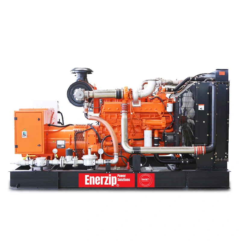
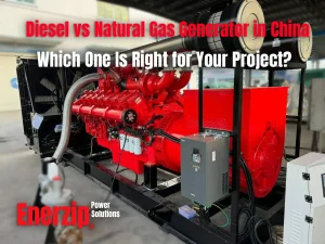
3) Fuel strategy: diesel vs natural gas vs biogas
- Diesel: strong transient response and robust standby behavior; storage/logistics and fuel quality management affect lifecycle outcomes.
- Natural gas: attractive for frequent operation when supply is stable; gas pressure/quality and compliance scope must be specified.
- Biogas: ROI-driven waste-to-energy; lifecycle cost is sensitive to fuel conditioning, methane variability, and contaminant control.
Biogas-specific lifecycle items often missed: gas cleaning/conditioning (H2S, siloxanes), condensate management, ignition components maintenance, and fuel-quality monitoring alarms. These can materially impact downtime risk and maintenance cost over a 10-year service life.
Maintenance, spares, and serviceability
Maintenance is not only oil changes. It is the operational discipline that protects lifecycle cost. Hidden costs are often labor hours, access difficulty, spare-part uncertainty, and unplanned corrective maintenance.
1) Service intervals and planned downtime
Ask suppliers to state service intervals for your duty cycle. A standby site with short monthly tests is different from a frequent-backup site with hundreds of hours per year. Planned downtime must fit your operational tolerance.
2) Spares clarity: “cheap parts” can still be costly
- One-year consumables list (filters, belts, hoses, coolant, lubricants).
- Critical spares list (starter components, sensors, AVR/regulator spares, breaker parts).
- Recommended spare strategy by duty (standby vs frequent operation).
- Documentation: part numbers, interchange notes, and lead-time assumptions.
Clear spares routes and service access reduce industrial generator TCO by cutting corrective downtime and labor hours during routine service.
3) Serviceability: access is a real cost
In canopy or container systems, service clearance and component layout affect labor time. Put packaging scope into procurement documents—not only drawings—to avoid hidden lifecycle labor costs.
Reliability events that prevent downtime
Reliability is not a slogan. It is the probability the system performs during an outage event. Downtime risk is the most underestimated component of lifecycle cost.
Define the “moment of truth” events
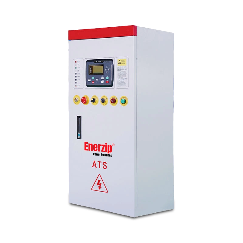
- ATS transfer and load pick-up timing (open vs closed transition, if applicable).
- Largest motor start after transfer (including re-acceleration behavior).
- Largest step load (UPS/rectifier pick-up, HVAC block, process block).
- High-ambient thermal stability (coolant temperature, enclosure temperature, airflow path).
Enerzip Field Note: For PLC/UPS-heavy industrial sites, practical acceptance targets are often stated (project must confirm with actual equipment tolerance): voltage dip ≤ 15% for ≤ 1–2 seconds during the worst motor start and frequency dip ≤ 10% with recovery within ≤ 5 seconds after the largest step load.
Verification habit: during testing, log load step size (kW/kVA), dip depth, recovery time, and the start sequence delay table used during the event. These measurable items shorten troubleshooting cycles later.
One big unit vs modular parallel
A single large genset is not automatically the safest option. Modular parallel architecture (N+1 optional) can improve step-load acceptance and allow maintenance without a full outage of backup capacity. This can lower lifecycle cost when downtime is expensive or future expansion is likely.
Controls scope (ATS/shedding/paralleling) and lifecycle cost
Controls scope is a major lever of lifecycle cost. Many “cheap” projects become expensive because the control boundary was unclear: who supplies staged load pick-up, load shedding, and protection coordination?
Integration boundary (who supplies what)
- EPC scope: load list, site SLD, cable sizing, grounding plan, ATS placement, and overall coordination.
- Genset supplier scope: controller logic, start sequence proposal, shedding tiers (if included), testing plan, and documentation pack.
- Switchgear/ATS vendor scope: ATS/switchboard hardware ratings, interlocks, protection, and interface wiring.
If this boundary is not written into the RFQ, the project often pays twice: once in procurement and again in commissioning rework.
Load shedding reduces size and improves stability
- Tier 1: must-run safety and controls.
- Tier 2: delay-start loads (pumps, compressors, staged HVAC).
- Tier 3: shedable non-critical loads.
Monitoring and event logs reduce troubleshooting cost
Remote monitoring, alarm history, and event logs reduce troubleshooting time after a trip—lowering maintenance labor and protecting lifecycle outcomes, especially in remote or multi-site deployments.
High ambient derating and poor airflow design can inflate industrial generator TCO through thermal trips, derated output, and repeated commissioning work.
Derating & cooling: the hidden cost multiplier
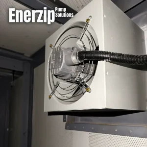
A generator stable in a factory may fail at site due to high ambient temperature, altitude, airflow restriction, dust, or enclosure recirculation. These are not minor details—they are major drivers of downtime risk and lifecycle cost.
High ambient: thermal margin is a system property
In 40–50°C regions, cooling system and airflow path become limiting factors. If thermal margin is insufficient, the unit may derate, alarm, or shut down during long runs.
Enerzip Field Note: A practical SAT record that improves troubleshooting: coolant temperature at stable load, enclosure internal temperature, and radiator inlet/outlet air temperature during a representative run. If problems occur later, these records help determine whether the limiting factor is load, controls, or airflow/recirculation.
FAT/SAT acceptance testing: buying fewer surprises
Acceptance testing converts marketing claims into verifiable performance. When procurement links system requirements to FAT/SAT scope, projects experience fewer surprises and lower lifecycle cost.
FAT (Factory Acceptance Test): what matters
- Visual inspection and wiring verification.
- Protection and alarm checks (over/under V & Hz, overspeed, E-stop).
- Control logic checks (start/stop, cooldown, ATS interface where applicable).
- Optional staged load steps to evaluate voltage/frequency dip and recovery (when required).
SAT (Site Acceptance Test): what proves real readiness
- Transfer behavior: utility-to-generator and re-transfer logic.
- Staged start sequence and load shedding validation.
- Worst-case event test aligned with your site’s “moment of truth.”
- Thermal verification under representative site conditions.
Worked example: low-price vs project-grade
This example shows how lifecycle cost changes when you include fuel, maintenance, and downtime risk. It is not a universal price table. Your real numbers depend on duty cycle, fuel price, and downtime value.
Assumptions:
- Service life: 10 years
- Runtime: 600 hours/year (frequent backup + testing)
- Average electrical load: 60% of rated kW
- Downtime value (conservative placeholder): USD 2,000/hour
- Acceptance targets defined in RFQ and verified via SAT
| Category | Low-price approach | Project-grade approach |
|---|---|---|
| CAPEX | Lower purchase price; scope gaps often remain | Slightly higher; scope defined (controls/testing/docs) |
| Fuel cost impact | Often higher due to oversizing/poor partial-load behavior | Optimized sizing + staged pick-up improves real consumption |
| Maintenance & spares | Unclear spares route; longer corrective downtime | Defined spares list + serviceability planning |
| Commissioning rework risk | Higher (ATS/motor start/airflow not defined) | Lower (FAT/SAT aligned with acceptance targets) |
| Downtime risk | Higher probability of nuisance trips | Reduced risk via controls + verification |
Numeric closure:
If Proposal A burns only 0.8 L/h more fuel than Proposal B at the site’s typical operating point, the 10-year fuel difference is:
ΔFuel (10y) = 0.8 L/h × 600 h/year × 10 years = 4,800 liters.
If diesel price is USD 0.9–1.3/L, then ΔFuel cost ≈ USD 4,320–6,240.
If unclear controls/testing cause just one avoidable outage event of 3 hours over the life, at USD 2,000/h, that’s USD 6,000—often larger than the purchase-price gap. This is why lifecycle cost decisions beat “lowest price wins.”
Use the checklist below to request the same data from every supplier so you can compare industrial generator TCO on a consistent basis.
RFQ-ready TCO checklist
Copy/paste into your RFQ:
RFQ — Total Cost of Ownership (TCO) Inputs
- Duty cycle: standby-only / frequent backup / prime; annual runtime hours; longest continuous run; average load factor.
- Fuel data: consumption at 25/50/75/100% load; basis conditions; whether figures include parasitic loads.
- Maintenance: service intervals; one-year consumables list; critical spares list; estimated lead times; service access requirements.
- Reliability events: define “moment of truth” events (ATS transfer, largest motor start, UPS step load, thermal run).
- Controls scope: ATS interface, staged load pick-up plan, load shedding tiers, paralleling/synchronizing scope, monitoring/event logs.
- Site conditions: design ambient & peak ambient; altitude; enclosure/container airflow constraints; dust/humidity/corrosion risks.
- FAT/SAT: propose acceptance test scope aligned with events; provide compliance matrix and assumptions.
Supplier response format: Compliance matrix (Comply/Deviate/Optional/Not included) + assumptions + datasheets + drawings + fuel curves.
FAQ
1) Is TCO only for prime power projects?
No. Even in standby applications, lifecycle cost matters because failures occur at the worst moment. Commissioning rework, poor transfer behavior, and thermal trips can cost more than fuel in the first years—especially when outages are rare but high impact.
2) What’s the fastest way to reduce lifecycle cost without buying a bigger unit?
Define staged load pick-up and load shedding tiers, then verify the “moment of truth” events through FAT/SAT planning. This improves stability and reduces nuisance trips without simply upsizing nameplate capacity.
3) How do I compare fuel numbers fairly?
Ask for fuel consumption at 25/50/75/100% load with clear basis conditions, then compare the same load point. Confirm whether figures include parasitic loads (fans/pumps) and be consistent about the measurement basis.
4) Do I need N+1 paralleling to reduce lifecycle cost?
Not always. Paralleling helps when downtime is expensive, step loads are large, or future expansion is likely. For smaller or simpler sites, a single well-integrated system with staged starts and verified acceptance targets may deliver the best lifecycle cost.
Next step
If you share (1) your load list (Excel), (2) duty-cycle intent (standby vs frequent operation), (3) site ambient/altitude and enclosure constraints, and (4) ATS/control scope requirements, Enerzip can help convert your inputs into a project-grade configuration and a supplier comparison matrix—so you can make a decision on lifecycle cost, not only purchase price.
Related resources
- How to Size an Industrial Backup Generator (kW vs kVA, ESP/PRP)
- Generator Specification Checklist for EPC Projects (RFQ-ready)
- Genset FAT/SAT Testing & Inspection Steps + Warranty Support
- Diesel Generator Sets
- Natural Gas Generator Sets
- Biogas Generator Sets
- Automatic Transfer Switches (ATS)
Note: This guide is an engineering workflow reference. Final requirements and acceptance targets should be confirmed against local codes, site drawings, equipment tolerances, and the agreed FAT/SAT scope.